TLDR: Used a Network model to evaluate all head to heads for each runner in the NAIA to generate a ranking for them. This system uses margin of victory over an opponent rather than time. Biggest draw back of this method is you can’t factor for bad races, tempoing a race, etc. I have provided a larger write up of the methods at the bottom.
The model has really punished anyone who ran at Gans Creek, as Spring Arbor beating many people there, but then running relatively even with Goshen at Bethel pushed all those teams down. Anyone who didn't run at Louisville avoided this. I might even redo the rankings to exclude the Bethel meet entirely--but it's hard to judge the "effort level" at any given meet.
At this point I don't consider these rankings much more than a novelty but I am open to suggestions if anyone has ideas on accounting for meets to exclude or how to more appropriately rank the individual runners. The model will likely do much better at predicting a nationals scenario as more crossover is generated with the regional races this week and then conference championships.
NAIA Men’s Great Lakes Model Predictions:
Team Score
Rio_Grande 50
Shawnee_State 85
Olivet_Nazarene 115
Campbellsville 146
Indiana_East 165
Indiana_Wesleyan 171
Spring_Arbor 179
Marian_IN 193
Taylor 205
Grace 224
Aquinas 263
Lawrence_Tech 273
Goshen 283
Cornerstone 344
St_Francis_IL 420
Governors_State_University 511
Indiana_Tech 520
Lindsey_Wilson 526
Madonna 534
Ave_Maria 534
Missouri_Baptist 556
Carroll_MT 576
Rocky_Mountain 590
Montana_Tech 660
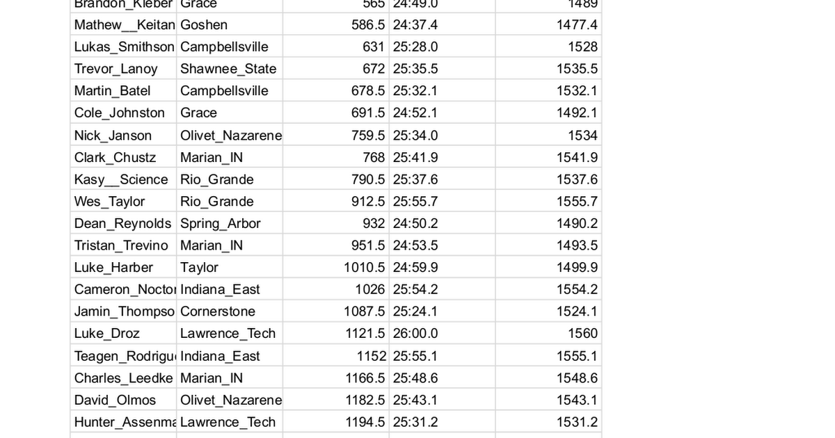
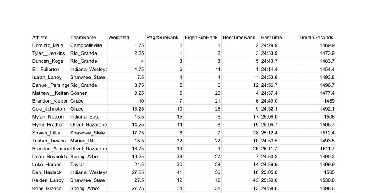
Athlete TeamName Weighted BestTime TimeInSeconds
Tyler__Jenkins Rio_Grande 147.5 24:33.9 1473.9
Dominic_Malel Campbellsville 173 24:29.9 1469.9
Duncan_Kogei Rio_Grande 227.5 24:43.7 1483.7
Isaiah_Lanoy Shawnee_State 251.5 24:53.8 1493.8
Danuel_Persinger Rio_Grande 294 24:56.7 1496.7
Shawn_Little Shawnee_State 384 25:12.4 1512.4
Eli_Fullerton Indiana_Wesleyan 385 24:14.4 1454.4
Mylan_Nocton Indiana_East 430.5 25:06.0 1506
Flynn_Prather Olivet_Nazarene 453 25:06.7 1506.7
Brandon_Armendarez Olivet_Nazarene 496 25:11.7 1511.7
Kaiden_Lanoy Shawnee_State 533 25:30.8 1530.8
Brandon_Kleber Grace 565 24:49.0 1489
Mathew__Keitany_ Goshen 586.5 24:37.4 1477.4
Lukas_Smithson Campbellsville 631 25:28.0 1528
Full Individual Ranking:
METHODS:
Use a Networks model to objectively rank each NAIA runners performance by analyzing any meet in which an NAIA runner participated in since 8-31-2024, assuming it was loaded to TFRRS. 154 as of today. This data includes 11,292 runners across all divisions.
Part 1: Match ups
This model generates each unique head to head matchup every runner was involved in during the year.
EXAMPLE:
Meet: Gans Creek 9-21-2024
Runner1: Ethan__Barker vs Runner2: Matt_Schieber
Margin of Victory : 5.5 (Positive Implies Victory for Runner1)
Meet: Seminole Valley 10-05-2024
Runner1: Ethan__Barker vs Runner2: Matt_Schieber
Margin of Victory: -5.6 (Negative Implies Victory for Runner2)
Part 2: Calculated Margin of Victory
Next generate a calculated amargin of victory for each runner against all of his opponents. This margin of victory was weighted so that more recent results hold greater value. While a standard average would show Matt_Schieber over Ethan__Barker by .05 seconds, this model uses a Time Decay Average Margin of Victory of .76 as Matt beat Ethan at their most recent race. This can be interpreted that you would expect Matt to beat Ethan by .76 seconds.
EXAMPLE:
Runner1: Ethan__Barker vs Runner2: Matt_Schieber
Standard Average Margin of Victory: -.05 (Negative Implies Victory for Runner2)
Time Decay Average Margin of Victory: -.76 (Negative Implies Victory for Runner2)
Part 3: Directed Graph
The graph network will have a single node, represented visually as a dot, for each runner in the results database. We now construct an edge, represented visually by a directional line, pointing from the slower runner to the faster with a weight value of “Time Decay Average Margin of Victory”. The weight value can be conceptualized as the thickness of the line. Runners who are relatively similar will be connected by a thin line, while runners with disparity will be connected by a thick line. This results in a graph with 11,292 nodes representing all individual runners, each with approximately 100 to 1500 incoming or outgoing lines connected to runners they have competed against. If the line is pointing into the runner, it indicates they are superior. If the line points to a different runner, that means the original runner is inferior.
Part 4: Ranking Algorithm
Next generate a ranking with the PageRank algorithm, using the thickness of the arrow to weight the results. Second create a separate ranking using Eigenvector Centrality. Create a composite ranking to be used as the final ranking by:
FinalRank = PageRank_Rank *50% + Eigenvector_Centrality_Rank *50%.
Part 5:
Order the Runners by FinalRank. Best time is provided only as a reference.